How can Data Science benefit from Software Engineering

About ten years ago, Harvard Business Review coined Data Scientist "the sexiest job" of the 21st century. Ever since the field has experienced an influx of new joiners from all backgrounds: Social scientists solving complex sociological dilemmas, mathematicians intrigued by the practical applications of statistics, or Computer Scientists interested in building cutting-edge features based on rich data.

But wait, what exactly is Data Science

Data Science remains a broad and, therefore, vaguely defined field. So, in this blog post, we will focus on Data Scientists who write Machine Learning code, which in comparison, finds a narrower description, as demonstrated by IBM's definition:

Machine learning is a branch of artificial intelligence (AI) and computer science which focuses on the use of data and algorithms to imitate the way that humans learn, gradually improving its accuracy.

While diversity drives innovation, a heterogeneous field of practitioners toughens the introduction of best practices. After all, the daily challenges of a political researcher investigating voting patterns diverge strongly from a development team fine-tuning face recognition techniques for your smartphone.
Where does this lead us as engineers, either working on a Data Science task or interacting with code that has to meet the requirements of scalable production code? Often with a disconnect between domain/ statistics expertise and best practices in Computer Science.

So, why should we care?

Data Scientists have successfully contributed to some of the most exciting inventions of the last decades - and many Data Scientists within IT departments already utilize the toolset of software engineers.

Nevertheless, many researchers, especially the ones not trained as traditional Software Engineers, might even be oblivious to the streamlined approach many IT projects follow. Writing tests, scaling code for high user numbers, outsourcing computing powers to cloud servers, documenting the work, or code modularization represent just a few examples that might make the life of a Data Scientist easier.

But while abstract concepts are excellent in theory, let us tackle a simple problem in two ways: First, how a small team of Data Scientists might explore a common problem. Second, re-approaching the same challenge as a Software Engineer, keeping some best practices in mind.

Let us look at it in action - two case studies

We will illustrate the diverging approaches with a simple prediction task: Given two exam scores, how likely a student is to pass or fail a given class.

The data

The data includes 100 observations, with two exam scores between 0 and 100 and one binary indicator of passing or not. The data is entirely made-up and allows for some predictability without being a fully deterministic indicator (for example, a summed score of 170 leads to passing the class).

The setup

We will use a typical setup for Data Science and solve this task in Python, the go-to tool for data science due to its popularity, ease of use, and extensive library universe geared towards data science. We will also solve the problem in a Jupyter Notebook for the data scientist, allowing a detailed description alongside the code. This notebook style combines the line-by-line rendering of R - another popular choice in Data Science - with inline visualizations and direct documentation.

Approach 1: The Data Scientist

Nice, let us get into the code! Wherever necessary to follow along, optional statistical or Data Science-related asides will ensure we are all on the same page to understand the problem. But do not worry - we keep the statistics hammering to a minimum.

First, we need to load the data:

path = './data/exam_data.txt'
data = pd.read_csv(path, header=None, names=['Exam 1', 'Exam 2', 'Pass'])
data.head()
data.shape()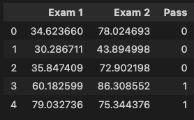

We can see the first five observations of the data and the overall shape of the data: (100, 3).

Training and testing the data on the same observations lead to unrepresentative self-fulfilling prophecies, so we need to split the data into training and test data sets - we will aim for a standard 80:20 split.

training = data[:80]
test = data[80:]

So let us examine the data a bit - how are passing students' test scores distributed in comparison to failing ones:

positive = training[training['Pass'].isin([1])]
negative = training[training['Pass'].isin([0])]

fig, ax = plt.subplots(figsize=(12,8))
ax.scatter(positive['Exam 1'], positive['Exam 2'], s=50, c='b', marker='o', label='Pass')
ax.scatter(negative['Exam 1'], negative['Exam 2'], s=50, c='r', marker='x', label='Not Pass')
ax.legend()
ax.set_xlabel('Exam 1 Score')
ax.set_ylabel('Exam 2 Score')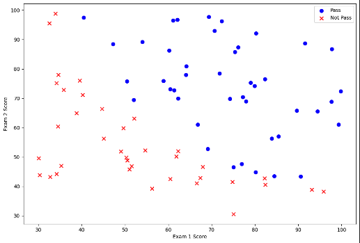

This visualization gives us the first hint that there might be some relationship between the two exam scores individually and towards the dependent variable, i.e., the student passing or failing.

But how to best quantify this notion? We will use a logistic regression model to predict whether students pass the class based on the exam scores.
Oh, oh, statistics...

Laying out the detailed derivation of the model will bore you and will not contribute much to the overall intent of the blog post. Just take the following building blocks with you, so the general approach is straightforward: we try to model a complex interplay of factors with a simplified representation of reality. This building block is called a model. In our case, we choose a mathematical relationship that helps us to translate continuous input variables, as in exam scores, to a binary (yes or no) outcome; this building block is called a logistic regression.

For our model to learn from data, we will use the toolset of Machine Learning, which over many iterations of observations, helps us to understand how important the exam scores are for the probability of passing the class. We call that finding the parameter weights of the input features.

To iterate over the data, we use a Gradient Descent approach that minimizes some cost function - a descriptor of the discrepancy between predicted and actual outcomes - leading us to optimal model parameters.

Let us look at the actual code. We can now define our gradient function to iterate through the data and - for the sake of simplicity - leverage a popular Python library to update the model parameters using the gradient function we define as:

def sigmoid(z):
    return 1 / (1 + np.exp(-z))

def gradient(theta, X, y):
    theta = np.matrix(theta)
    X = np.matrix(X)
    y = np.matrix(y)

    parameters = int(theta.ravel().shape[1])
    grad = np.zeros(parameters)

    error = sigmoid(X * theta.T) - y

    for i in range(parameters):
        term = np.multiply(error, X[:,i])
        grad[i] = np.sum(term) / len(X)

    return grad

Given the gradient function, we can optimize the model parameters (the weights given to the two test scores) with SciPy:

import scipy.optimize as opt

result = opt.fmin_tnc(func=cost, x0=theta, fprime=gradient, args=(X_training, y_training))
result

So, this is it. We are done. We have found an optimal model to predict students' passing or failing based on the two exam scores. But wait, how well are we doing? We will need a predictor function to run on the test data set to determine that:

def predict(theta, X):
    probability = sigmoid(X * theta.T)
    return [1 if x >= 0.5 else 0 for x in probability]

We can see that we run a set of observations (only the X values, though, therefore, only the exam scores) through our sigmoid function and then make a hard cut-off above or below 0.5 probability to predict passing or not. We can then compare these values to the actual Y values we had in the data for these observations to see how accurate our predictions were:

theta_min = np.matrix(result[0])
predictions = predict(theta_min, X_test)
correct = [1 if ((a == 1 and b == 1) or (a == 0 and b == 0)) else 0 for (a, b) in zip(predictions, y_test)]
accuracy = (sum(map(int, correct)) % len(correct))

This model correctly predicts 90% of observations within the previously unseen test data set.

Approach 2: The Software Engineer

So far, we have read a good bit about how a data scientist tackles a classification problem, have been reminded of long-dreaded university-level statistics, and have yet not covered anything this blog post promised: How to marry data science and software engineering's best practices.

The detailed explanation was necessary, though, to better comprehend the complexity of decisions made by a data scientist.

While many engineering problems can take one of two or three routes, data scientists must select (and often first test) from a vast universe of possible tools in their kit.

Therefore, thoroughly understanding some of the methods to solve the problem will become valuable when deciding on a target architecture for code modularization - unfortunately, there is no one-size-fits-all solution.

What is different?

Software engineers have to think of scalability. Therefore, we will refrain from the Jupyter notebooks and instead work in modularized Python files, defining classes for the different stages of the analysis:

1. Data loading
2. Data cleaning/preparation
3. Exploratory analysis
4. Regression analysis
5. Prediction/Model evaluation

To make the steps within this post crystal clear, we will work overly granularly and create Python classes for every single step. In a real production scenario, it probably makes sense to bundle multiple actions together.

How to organize the code?

Code modularization has come up several times in this text, but what does it mean? Remember the single-file approach of the eager Data Scientist? While this technique works well for some quick and dirty drafts or small result presentations, it fails to address general concerns of production-ready code. Look at the folder structure of the same problem we faced earlier in a more extendable hierarchy.:

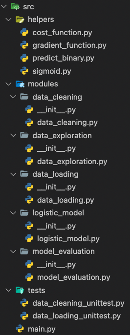
Why would we want to extend our nice single Jupyter notebook to this abomination of a project? Because it nicely separates code into distinct components!

Let us look at it step by step; the main magic happens in the main.py file, which calls all other files to do certain functionalities. So, for example, to load the data from an arbitrary backend server, or in our simplified case, from a local file, we call:

from modules.data_loading.data_loading import DataLoading

loader_instance = DataLoading('./data/exam_data.txt')
DataLoading.load_data_to_pd(loader_instance, None, ['Exam1', 'Exam2', 'Pass'])

Easy, right? We can achieve this behavior because, as Software Engineers, we have extracted the unorganized cells of the notebook into consolidated Python classes:

import pandas as pd

class DataLoading:
    """Class to load the data from an arbitrary path

    Args:
        path (string): String argument that holds the path (web or local) to load the data - here just for .csv files - can be extended to other file types
    """

    def __init__(self, path) -> None:
        self.path = path
        self.data = None

    def load_data_to_pd(self, header: bool, names: list[str]):
        """This method loads the data into a pandas dataframe object.

        Args:
            header (bool): Indicator if the pandas dataframe will load data including a header or not
            names (list[str]): List of column names
        """
        self.data = pd.read_csv(self.path, header=header, names=names)

    def showcase_pd_data(self, number_of_items: int):
        """Helper function to show the first entries of the data and its actual shape.

        Args:
            number_of_items (int): Number of items to be shown by the preview
        """
        print(f'Data shape is: {self.data.shape}')
        print(self.data.head(number_of_items))

This approach allows us to synergize all related functionality under one roof, document it accordingly, and even write dedicated unit tests in a separate file:

import unittest

from modules.data_loading.data_loading import DataLoading


class TestDataLoading(unittest.TestCase):
    """
    Test Class for the Data Loading process
    """

    def test_load_data_to_pd(self, path, header, column_names):
        """Test method for the actual loading of data. It asserts the loaded
        data shape against expected dimensions.

        Args:
            path (str): Path to the data to be loaded
            header (bool): Input variable to indicate wheter the loaded data includes a header
            column_names (list[str]): Array of the columns included in the data
        """
        loader_instance = DataLoading(path)
        loader_instance.load_data_to_pd(header, column_names)
        loaded_data = loader_instance.data
        self.assertEqual(loaded_data.shape, (100, 3),
                         'Data shape should be (100,3)')

We can quickly see how extending the data loader to different input formats, dynamically retrieving data from a backend (including passing on tokens or other identification), or even formatting it into something other than pandas, means extending the existing class.
Software programs in production are rarely static but often a collaboration of many people. Therefore, predicting how large or complex a seemingly small feature will eventually become is almost impossible. I would rather err on overthinking than start from scratch because quick and dirty did not cut it.

Let us compare one more example of what code can look like in a more scalable version:

import numpy as np

class DataCleaning:
    """The class to clean the loaded data.

    Args:
        raw_data (pandas df): The actual data to be split into train and test data and to be cleaned.
    """

    def __init__(self, raw_data) -> None:
        self.raw_data = raw_data
        self.training_data = None
        self.test_data = None
        self.X_training = None
        self.y_training = None
        self.X_test = None
        self.y_test = None
        self.theta = None

    def create_training_test_split(self, training_proportion: float):
        """Method to split the data into test and training data according to a pre-specified proportion.

        Args:
            training_proportion (float): The proportion of the data to be used for training the model.
        """
        self.training_data = self.raw_data[:int(
            training_proportion * len(self.raw_data))]
        self.test_data = self.raw_data[int(
            training_proportion * len(self.raw_data)):]

    def prepare_data_log_regression(self):
        """The data needs to be prepared to be appropriately consumed by the model function. Here we create
        the feature matrix X of shape(# of observations, # of features) and the result vector y of shape
        (# of observations, 1)
        """
        self.training_data.insert(0, 'Ones', 1)
        self.test_data.insert(0, 'Ones', 1)

        cols_training = self.training_data.shape[1]
        cols_test = self.test_data.shape[1]
        self.X_training = self.training_data.iloc[:, 0:cols_training-1]
        self.X_test = self.test_data.iloc[:, 0:cols_test-1]
        self.y_training = self.training_data.iloc[:,
                                                  cols_training-1:cols_training]
        self.y_test = self.test_data.iloc[:, cols_test-1:cols_test]

        self.X_training = np.array(self.X_training.values)
        self.X_test = np.array(self.X_test.values)
        self.y_training = np.array(self.y_training.values)
        self.y_test = np.array(self.y_test.values)

    def initialize_parameter(self):
        """Initialize our theta vector that will eventually hold the parameter weights optimized in the model
        """
        self.theta = np.zeros(self.X_training.shape[1])

This slightly longer class includes all the necessary steps for us to wrangle the data and prepare if for the upcoming modeling steps. We have a clear separation of concerns between the simple functionality to split the data set into training and test data, reshaping its dimensions for the vector operations, and initializing our parameter vector theta.

Testing these methods becomes much more accessible and will be naturally well-documented. Important to distinguish here are software tests of training and inference code: Training code tests fall under the responsibility of the Machine Learning practitioner - how does the model run, where can we fine-tune parameters, etc.? The more poignant side of the coin will be how inferences impact the product and user experience. Therefore, streamlined standards for these tests will ensure the quality and maintainability of the code base.

These functionalities go hand in hand with the usual benefits of modularized Python projects, such as virtual environments with a clearly defined dependency management via a pyproject.toml file.

Where does that leave us, and what to do from here?

We have explored how Data Science has become one of the professional trends of the 21st century that will not fade away anytime soon. While it has brought remarkable technological advances, its diverse problem space creates a conundrum of best practices to follow.
I propose that Software Engineering's approach to problems proves useful for Data Scientists aiming for scalable and testable production-level code.

The main benefits, which I tried to illustrate along a simple classification problem, are that:

• modularized Python code is more straightforwardly maintained, explored, and collaborated on
• distinct classes with often a singular purpose can be tested and extended easily (in comparison to prevalent notebook approaches in Data Science)
• you never know how and when a model will become more complex. We could even split up our toy example into five sequentially operating modules. These steps allow for many other approaches to retrieving the data, which model to apply, and how to benchmark it. Our system enabled easy extensions for feasible alternatives

Let us assume we find N/A values in our data and would like to add a pre-processing step to the data-cleaning pipeline. In a Jupyter Notebook, this would require us to be aware of the state of the currently loaded data (did we already remove the N/A's?) and find the best spot to include this additional step. In our modularized approach, we can add a single method to the DataCleaning class that checks for null values.

class DataCleaning:
    """The class to clean the loaded data.

    Args:
        raw_data (pandas df): The actual data to be split into train and test data and to be cleaned.
    """

    [...]

    def remove_null_values(self):
        """Method to remove null values from dataframe."""
        self.clean_data = self.raw_data.dropna()

Other alternatives would be model extensions as additional modules or more scaling/preprocessing steps when loading/cleaning the data.

There is a definite use case for prototyping in the Jupyter notebook, which proves especially useful in an introductory presentation of results to an uninformed audience.

But, if the goal is to build solutions to complex problems in teams that benefit from a predefined code quality, working in designated Python modules and following industry-proven Software Engineering principles will significantly help.

Footnotes

1. For the sake of the example, let us assume that these are test exams, which do not fully determine if a student passes by themselves. Otherwise, this would not be a statistical but a purely additive, i.e., deterministic exercise.↑

2. Technically, this so-called co-variance between the individual predictors is not ideal. We would want to add factors to our model that are highly explicative of the dependent variable but are agnostic (independent) of each other.↑

3. This approach might be overkill for this particular scenario of a quick logistic regression. But, if we wanted to compare multiple models, add tests for all helper functions, and see this as a starting point, a clear distinction between the functionalities within small-scoped classes might simplify the code.↑

4. Tests are added for the loader and cleaner classes for illustrative purposes. In a production-level scenario, one might consider writing the tests before the actual code, following the so-called TDD - Test-Driven-Development approach.↑

5. The alternative to classes would be stateless modules, which in this use case might even be more appropriate because our pipeline does not depend on any features for which software classes are beneficial - statefulness, hierarchical inheritance, etc. Still, classes, as a cornerstone of Object Oriented way to structure code, make this short introduction more accessible to the diverse background of software engineers not familiar with Python syntax or language-specific intricacies.↑

Published by Marc Luettecke

Visit author page