Comparing Fact Sheets using Graph Convolutional Networks

Why do we compare Fact Sheets?

Fact Sheets are the central element within LeanIX (What is a Fact Sheet?). As a result, many of our data science use cases rely on a machine-processable representation of such a Fact Sheet.
Recommending potentially interesting Applications or IT Components, for example, is a task that can be tackled by comparing Fact Sheets to previously viewed ones. Say a user is investigating database solutions and has looked at Oracle and PostgreSQL. We may want to recommend that they also look at MongoDB (assuming the IT Component exists in the workspace).

Fact Sheets on these database systems would ideally be more similar to each other than Slack (communication platform). Programmatically, this is a complex task, mainly due to the information-rich structure that makes up a Fact Sheet.

Fact Sheets as Graphs

Fact Sheets are used for documenting and saving information regarding architectural objects, like Applications, Business Capabilities, or IT-Components. They are rich in information as they combine attributes (e.g. technical and functional suitabilities) with relations to Fact Sheets of the same and other types.

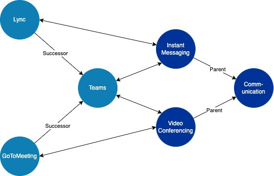
From a data processing point of view, graph structures are most suited to include all this information. Fact Sheets become nodes and their relations edges – both of which can have types and attributes. However, graphs per default are not comparable. There is no intuitive rule to determine a score of how similar two nodes in a graph are to one another.

GCNs to the rescue!

Graph Convolutional Networks are a family of neural networks that work directly on graphs to take advantage of all available information. Given one or more graphs a network is trained to solve one or more specific tasks.
With Fact Sheets, for example, we can classify by predicting each nodes type (Application, IT Component, Provider, ...). While the last network layer will be set up to output one of the types, the outputs of previous (also called hidden) layers are interpreted as numeric representations of a Fact Sheet. These vectors are what we call Fact Sheet embeddings.

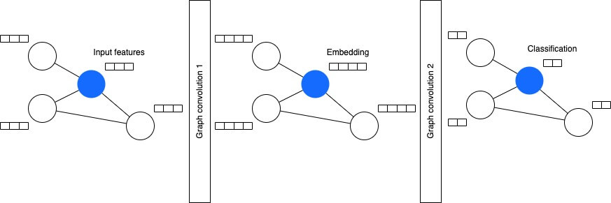
At its core, each graph convolution computes an aggregation (usually sum or average) of the features of the current node and its direct neighbours. This concept is called Message Passing. For the first convolution, the output for each node (Fact Sheet) is an embedding with mixed information from the node itself and its direct neighbours.

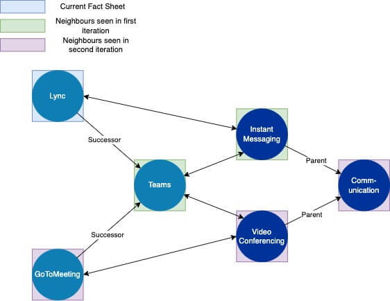
When stacking up convolutional layers, the resulting embedding of each Fact Sheet will be influenced by a larger portion of the overall graph.

Wait, there is more!

In its initial form, GCNs do not differentiate between different kinds of edges. With relational GCNs a set of dedicated weights is learned per edge type. This way a Predecessor/ Successor relation can have a different impact than an Application to Business Capability relation.

Besides node classification, GCN can be used for link prediction and graph embedding.
Using link predictions we can suggest edges that are missing from a graph. The neural network is constructed in the form of an auto-encoder. This way it reconstructs the graph given a latent factor representation. As a result, we can predict missing relations between Fact Sheets.

If how we embed Fact Sheets and GCNs in general sparked your interest make sure to check out the resources linked below!

Resources

• A Gentle Introduction to Graph Neural Networks
• PyTorch Geometric
• Semi-Supervised Classification with Graph Convolutional Networks
• Modeling Relational Data with Graph Convolutional Networks
• Variational Graph Auto-Encoders

Published by...

Philipp Glock

Visit author page

Sebastian Hätälä

Visit author page